Chapter 2 GIS basics

2.1 Datums, Projections, and Coordinate Systems

Datums

The Earth is a spheroid (also called an ellipsoid). Because of variations in elevation across the world, the Earth’s surface is irregular.

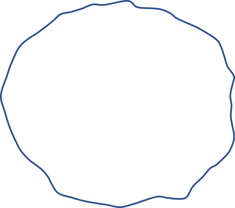
Figure 2.1: Conceptual representation of the irregular, spheroid shape of the Earth

A datum (also called a geographic coordinate system) is a reference surface that best fits the mean surface area of an area of interest. There is a global datum to represent the general surface of the Earth as a whole — World Geodetic System of 1984 i.e. WGS84.

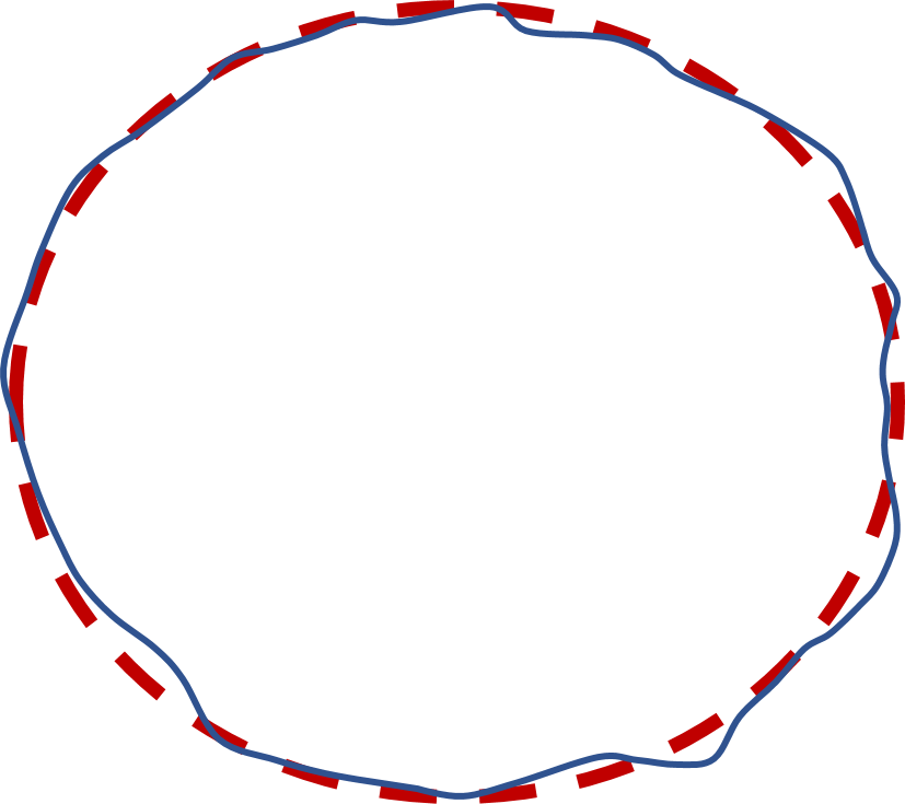
Figure 2.2: Red ellipse represents the smooth, general surface of the Earth (i.e. a global datum)

However, because the Earth’s surface is irregular and the global datum might not reflect specific areas and variations in elevations, there are also local datums. A common local datum (for North America at least) is the North America Datum of 1983 (NAD83) .

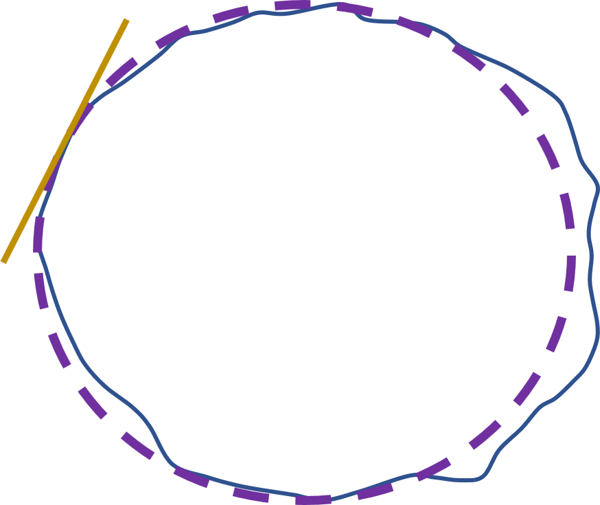
Yellow line indicates a specific area, purple ellipse represents the smooth, general surface of the Earth at this location. Note that this local datum would not be a best fit in other places on the Earth

Figure 2.3: Yellow line indicates a specific area, purple ellipse represents the smooth, general surface of the Earth at this location. Note that this local datum would not be a best fit in other places on the Earth

The datum you choose to work with is up to you and where your study takes place. It is very important to know what datum you’re working with and that you remain consistent because coordinates of a location from one datum are likely different than the same location from a different datum. For example, if we look at the coordinates for Bellingham, Washington:

Datum	Longitude	Latitude
NAD 1983	-122.46818353793	48.7438798543649
WGS 1984	-122.46818353793	48.7438798534299

While the differences between NAD83 and WGS84 are not huge, these differences could impact any spatial analysis you perform. Also note that you would need to choose a different local datum if you’re working outside of North America.

Projections

While a datum references the position of an object in geographic space on a 3D surface, a projection (also called a projected coordinate system) represents that 3D surface onto a 2D plane.

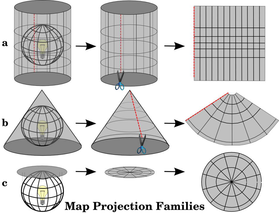
Figure 2.4: Conceptual demonstration of map projections

This is important to know when plotting a map for a figure, as your chosen projection will change the visualization and shape of your map’s features. But more importantly for spatial analysis, a projection is needed when you need values such as length, area, or distance. Map projections are never 100% accurate, so every 2D map will have show some distortion. Different projections preserve different properties of the world, such as the relative shape of features, area, distance, or angle. For that reason, it’s important to pick a projection that would provide the highest accuracy for your region and the analysis you’re running.

A common projection to use is the Universal Transverse Mercator or UTM.

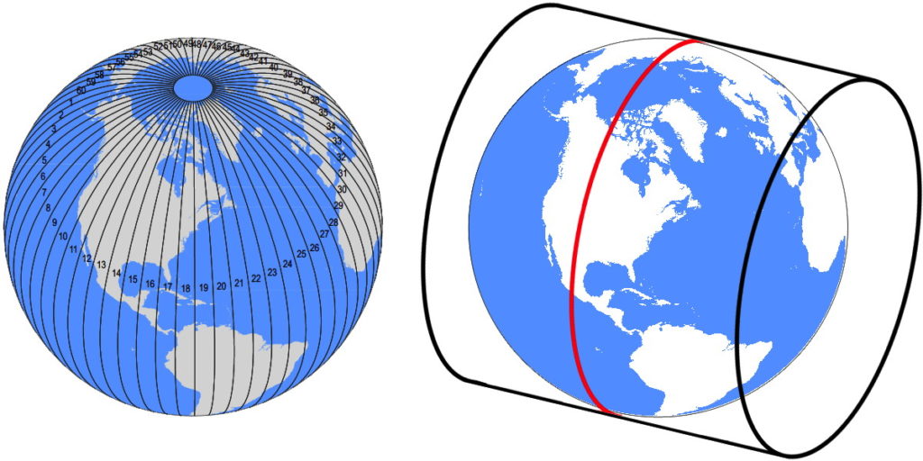
Figure 2.5: UTM around the globe

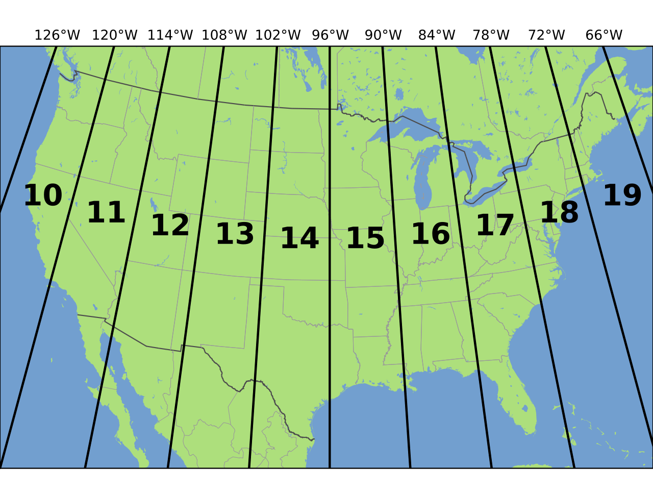
Figure 2.6: UTM for the US

If your study region is in Utah, for example, you would use UTM Zone 12 N (or UTM 12N).

Note that while you will always have a datum, you do not necessarily need to ALWAYS use a projection. As for anything, it depends on your analysis and your system.

Coordinate Reference System

A coordinate reference system or CRS is simply the combination of the datum (geographic coordinate system) and the projection (projected coordinate system). For example, if you are working with the 1984 World Geodetic System that is projected to UTM Zone 12N, your CRS would be WGS84 UTM12N. If you are working with the 1983 North America Datum that is projected to UTM Zone 14N, your CRS would be NAD83 UTM14N. And so on.

These different combinations of CRS all have their own EPSG code. (These codes were orginally created by the European Petroleum Survey Group, which is where the acronym comes from).

For example, the EPSG code for WGS84 latitude/longitude (i.e. no projection) is 4326, the EPSG code for NAD83 UTM12N is 26912, and so on. These codes can easily be found on the Spatial Reference Website (or google if you forget what the website is).

2.2 Spatial Data

Vectors

Vector data are shapes with a geometry that can represent real world features. These geometries which can be made up of one or more vertices and paths. A vertex describes a position in space with x and y coordinates. A feature with one vertex would be a point, a feature with two or more vertices where the first and last vertices don’t connect would be a polyline, and a feature with at least three vertices and the first and last vertices connect (an enclosed area) would be polygon. Here are some examples of vector data that you might encounter in ecology:

Points
- animal positional locations
- study site coordinates
- tree locations
Lines
- roads
- fences
- boundaries
- rivers
Areas (or polygons)
- bodies of water
- parks
- USFS land
- study plots
- area burned by a fire

Example with random vertices:

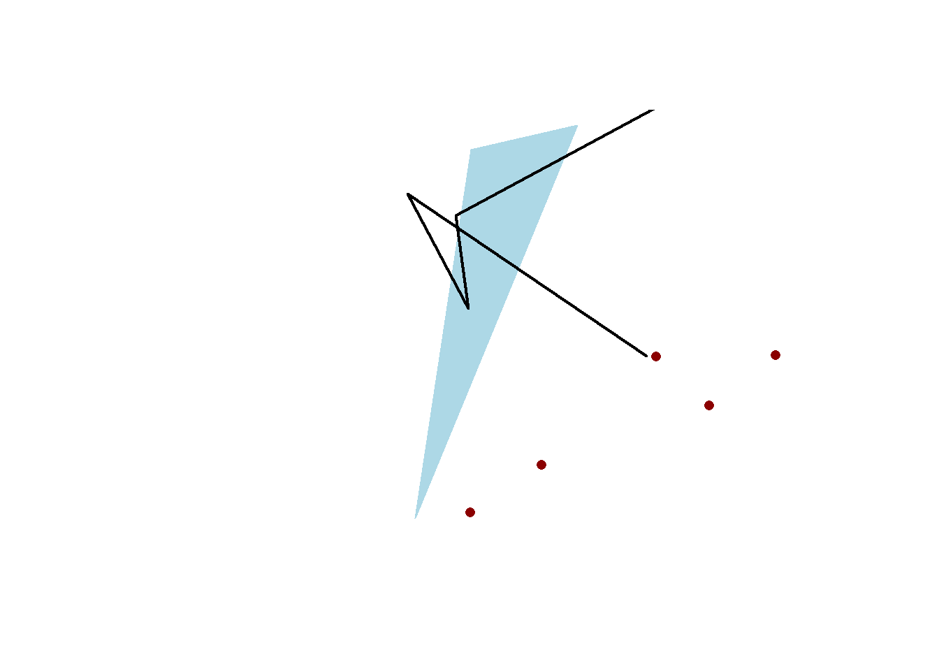
Figure 2.7: Figure demonstrating points (red), polylines (black), and polygon (blue)

Or an example with Utah features:

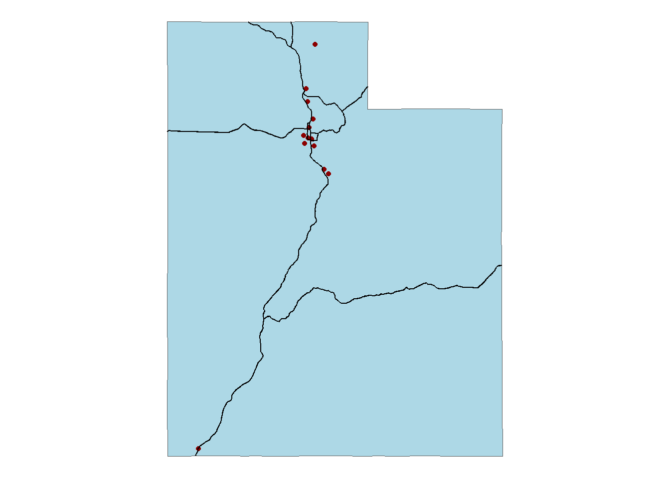
Figure 2.8: Figure demonstrating points (major Utah cities), polylines (major Utah highways), and polygons (shape of Utah boundary)

Vector features have attributes, which can be text or numerical information that describe the features. These attributes are stored in a data frame.

##                   name state    pop   lat    long capital
## 1         Bountiful UT    UT  41622 40.88 -111.87       0
## 2            Layton UT    UT  63096 41.08 -111.95       0
## 3             Logan UT    UT  45262 41.74 -111.84       0
## 4            Murray UT    UT  56848 40.65 -111.89       0
## 5             Ogden UT    UT  78572 41.23 -111.97       0
## 6              Orem UT    UT  94758 40.30 -111.70       0
## 7             Provo UT    UT 105832 40.25 -111.64       0
## 8      Saint George UT    UT  63952 37.08 -113.58       0
## 9    Salt Lake City UT    UT 177318 40.78 -111.93       1
## 10            Sandy UT    UT  89698 40.57 -111.85       0
## 11     Taylorsville UT    UT  58200 40.66 -111.94       0
## 12      West Jordan UT    UT 105629 40.60 -111.99       0
## 13 West Valley City UT    UT 113989 40.69 -112.01       0

Some important information you need from your vector data are:

the geometry type (if it’s a point, line, or polygon)
the coordinate reference system
the bounding box (the min/max points in x and y geographical space)

Rasters

Rasters are data represented by pixels (or cells) where each pixel has its own value. These cell values can be continuous (e.g. elevation, temperature, snow depth) or discrete (e.g. land cover, habitat type, presence/absence).

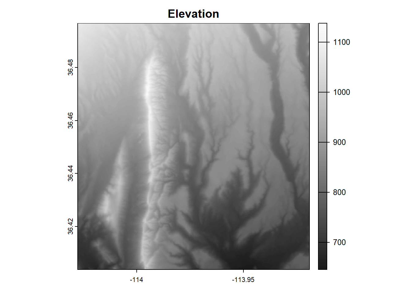
Figure 2.9: Map showing a raster with continuous values (elevation)

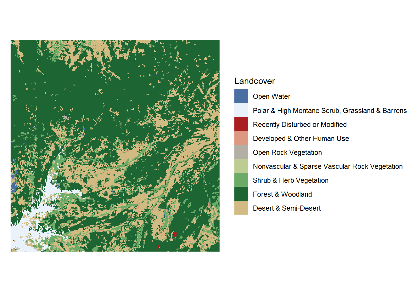
Figure 2.10: Map showing a raster with discrete values (land cover)

Raster data can have more than one band (where each band is a single raster). These raster layers can stack together to create a Raster Stack. For example, satellite imagery is a stack of 3 rasters, each containing continuous values indicating levels of Red, Green, and Blue.

## class       : SpatRaster 
## dimensions  : 1679, 2312, 3  (nrow, ncol, nlyr)
## resolution  : 0.0008983153, 0.0008983153  (x, y)
## extent      : -113.2237, -111.1468, 40.27956, 41.78783  (xmin, xmax, ymin, ymax)
## coord. ref. : lon/lat WGS 84 (EPSG:4326) 
## source      : landsat_demo.tif 
## names       : Red, Green, Blue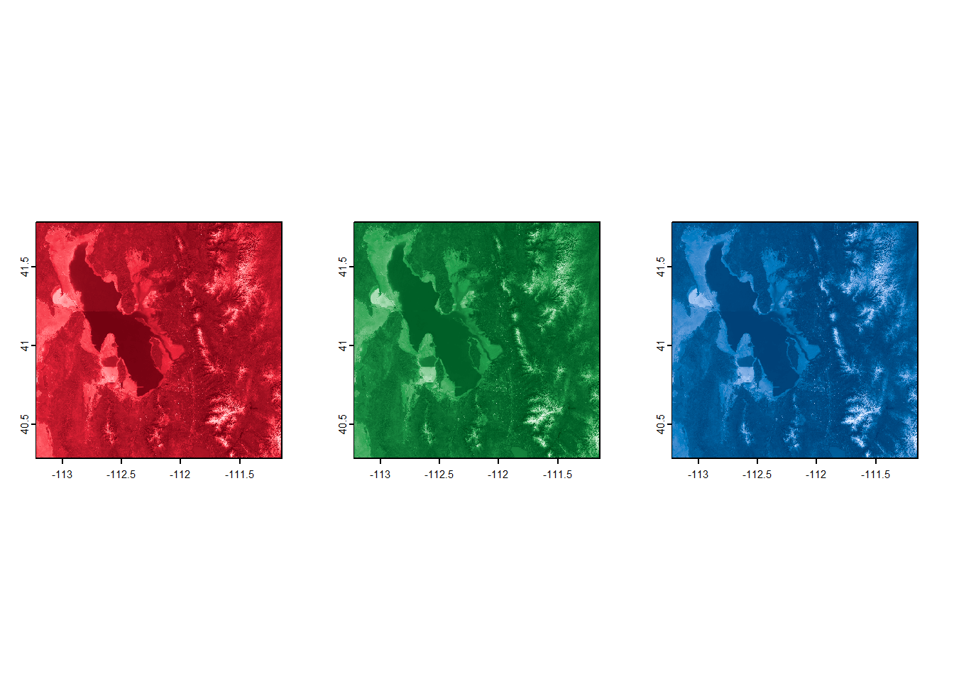

Figure 2.11: Plotting a single band of a satellite image will only show the individual values of RGB

But these 3 bands come together to make a true-color image.

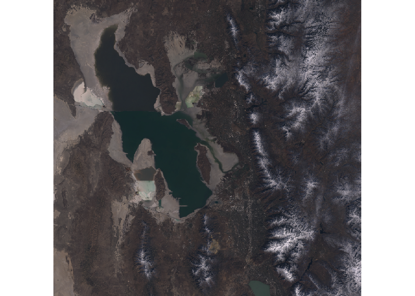
Figure 2.12: True-color satellite image of the Salt Lake region

The important information you need from your raster data are

the coordinate reference system
the extent (the min/max points in x and y geographical space)
the cell resolution (the width and height of each cell)

The cell resolution basically means how “pixel-y” the raster is. A finer resolution (meaning the cell size is smaller) will have more detail than a coarser resolution (meaning the cell size is larger). For example, compare a raster with a pretty fine resolution (in this case 30m X 30m, meaning that each cells is 30-m wide and 30-m high)

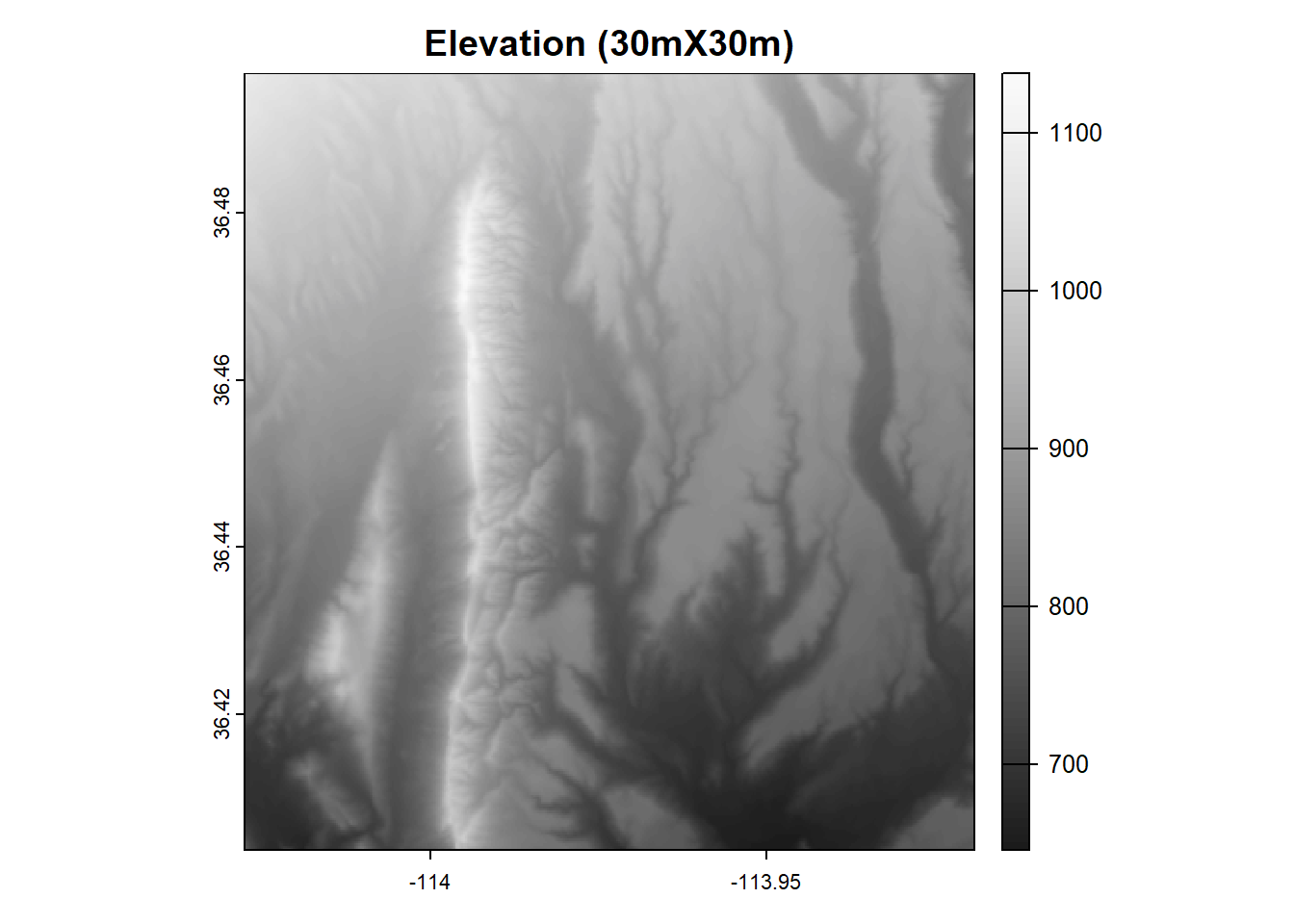
Figure 2.13: Map showing a raster with fine resolution (30m X 30m)

Compared to the same raster but with a coarser resolution (in this case 300 m X 300 m)

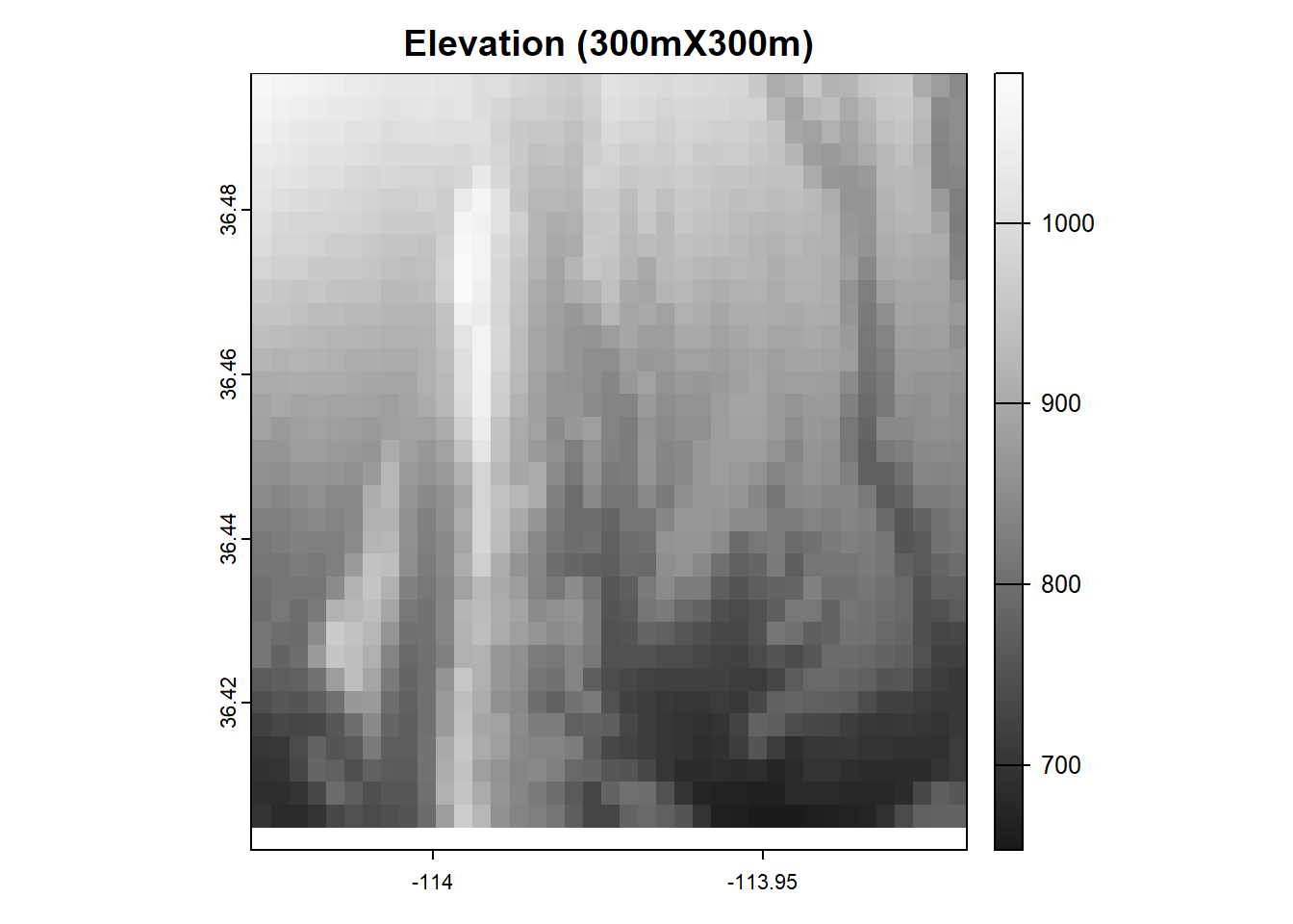
Figure 2.14: Map showing a raster with coarse resolution (300 m X 300 m)

Wouldn’t we always want to work with finer resolutions? If rasters with finer resolutions have more detail (and thus are more accurate to what’s actually on the landscape) than one with a coarser resolution, why would we ever work with a raster with coarse resolution? I can think of 2 reasons why:

Sometimes you simply can’t obtain that data in a finer resolution. For example, MODIS offers NDVI rasters every 16 days, but the finest resolution is 250-m.
The finer the resolution, the more cells there are, and so the time, computation power, and disk space to do any sort of computation or analysis on these cells increases.

As for everything, it depends on your analysis and your system.

2.3 Vectors vs Rasters: pros & cons

Advantages of Vectors

Because vectors are just vertices and paths (rather than upwards of millions of grid cells), it takes less time to load, save, or perform any computation or analysis on a vector compared to a raster. (They also take up less disk space on your hard drive)
For the same reason, they can often be more geographically accurate. A vector’s vertex is located at a single lat/long coordinate compared to a raster pixel at the same location but covers 250mX250m.

Disadvantages of Vectors

It is difficult to store and display continuous data in vectors. (It can be done, but the data typically would need to be binned)
Vectors are best used to represent features of the landscape, rather than the landscape itself.

Advantages of Rasters

Rasters are best for satellite and other remotely sensed data. As the point above mentioned, they are great for representing the landscape itself.
It is relatively easy and intuitive to perform any quantitative analysis with rasters. When raster cells are stacked (see figure below), it is pretty straightforward to perform any focal statistics or cell algebra.

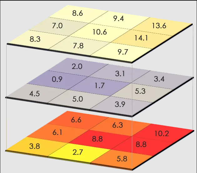
Figure 2.15: A stack of rasters, showing how each cell would correspond to the ones on top and below

Disadvantages of Rasters

Depending on the resolution, they can look pixellated and not visually appealing. For analysis, this would affect computation time and disk space.
Raster cells can only contain one value (compared to vectors, which can have an entire attribute table). If you want cells to contain more than one value, you would need a stack of rasters, which takes up disk space and computation power.

Now that we know about coordinate reference systems, vectors, and rasters, let’s learn how to deal with all of these in R!